The Central Limit Theorem is one of those spooky math results that probably keep mathematicians awake on full moon nights. This post will try and illustrate the central results of the theorem so that some of us slumbering mortals might also lose some sleep occasionally.

In essence the theorem states that given a bunch of numbers (aka the Population), if you randomly select small - but big enough - groups of numbers (aka sample) from it and add the numbers in these samples together; the group of numbers produced as a result of this addition will always be distributed in a specific pattern called the normal distribution. The addition component is very important, it’s not enough that you select samples from the population, you must add the data within the samples for the CLT to hold. This also means that whenever you are dealing with some data that could possibly be expressed as the result of randomly summing other quantities you can apply the CLT.

The cool part here is that even though you don’t know anything about the original population, you can find it’s mean and variance if you take a set of large enough samples.

Now if instead of just adding the numbers inside the samples, we calculate their average or mean, some more interesting results can be obtained. Lets also introduce some notation to make the textual statements clearer.

Population mean = $ \mu_P $, variance = $ \sigma_P $ (aka sample distribution)

Set of sample means = $\{ \mu_0 , \mu_1 , ... , \mu_N \}$ (aka sampling distribution)

Mean of set of sample means = $\mu_X$, variance = $ \sigma_X$

1. The mean ($ \mu_X $) of the set of sample means will approach the actual mean of the population
2. The variance ($ \sigma_X $) of this mean is approximately equal to the population variance divided by N ($ \sigma_P/N $), where N is the size of each sample (i.e. the count of numbers in each sample)

More about N

The sample size N is rather important, it must be reasonably big for the CLT to hold. If it’s too small, then there’s not going to be any soup for you. The right size of N depends on the original sample population. If the original population is a decent symmetric one then - according to the math gurus - a value of N <= 30 is good enough. However if the original population is skewed, then you might need higher values of N. For example imagine an impulse function - a value of K at one point and 0 elsewhere. You might need a large sample from the population to end up with a sample that has K inside it.

Proof or maybe not

Since the proof of a pudding is in the coding and not in the deriving, let try some experiments.

The below script calculates the Population and Sample statistics based on CLT, and plots a histogram of the sample means for a given population function. Feel free to play around with different settings for N and P. I use N = 40 as the threshold in the script, but 30 should also yield similar results.

1
2
3
4
5
6
7
8
9
10
11
12
13
14
15
16
17
18
19
20
21
22
23
24
25
26
27
28
29
30
31
32
33
34
35
36
37
38
39
40
41
42
43
44
45
46
47
48
49
50
51
52
53
54
55
56
57
58
59
60
61
62
63
64
65
66
67
68
69
70
71
72
73
74
75
76
77
78
79
80
81
82
83

# Central Limit Theorem Illustration

# THEOREM
# ==========
# Tells us that the sampling distribution of the sample mean is, at least approximately, 
# normally distributed, regardless of the distribution of the underlying random sample.
# The maean of this distribution of samples means is EQUAL to the population mean
# The variance of this (new) mean of distributions is EQUAL to the (population variance / N)
# [The error with respect to the population mean decreases as N increases]
# where N is the sample size
# NOTE:
# (1) The larger the sample size N, the smaller the variance of the sample mean.
# (2) If the underlying distribution is skewed, then you need a larger sample size, typically N > 30
#     for the results to hold
# (3) This is only applicable to the Mean, variances follow the Chi-squared distribution
#
# https://onlinecourses.science.psu.edu/stat414/node/177
# EXTRA:
# The sampling distribution of the sample variance is a chi-squared distribution with degree of 
# freedom equals to N−1, where N is the sample size
# The chi-squared distribution looks skewed compared to normal distribution
# http://onlinestatbook.com/2/chi_square/distribution.html
#

# population size
P = 50000
# sample size --> Increase this to getter closer to ideal results
N = 40
# sample count --> This is also important in practise
C = 1000



## ----- Setup the population ----
# Select any probability function and convert it to discrete form with P points

# (1) Exponential function - change the factor from 1 - 100 to increase skew
# Sequential sampling of the PD function
pd = exp(seq(from = 0.0, to = 10.0, by = 10.0/P))
# Random sampling of the PD function
#pd = exp(runif(P, 0.0, 10.0))

# (2) Ramp function
#pd = seq(from = 0.0, to = 10.0, by = 10.0/P)

# (3) Sine function
pd = sin(seq(from = 0.0, to = 2*pi, by = 2*pi/P))

# (3) Random function
pd = runif(P, 0, 10^12)

# Allocate a matrix to hold the sample data
s = matrix(0,C,N)

## ----- Take C samples of same size from the population ----
for (i in 1:C) {
  # Create a matrix of random indices with sample size
  idx = matrix(sample(c(1:P), size = N, replace = TRUE))
  # Select random samples from our probability function
  s[i,] = pd[idx]
}

# Now s[] contains C samples from the population pd
# Lets do some statistics on the samples

par(mfrow=c(3,1))
plot(pd,main="Population function")
## MEAN
# prob TRUE converts the counts into probability and is necessary to draw the density function overlay
hist(rowMeans(s), plot = TRUE, main = sprintf("Histogram of sample means (N=%i)", N), prob=TRUE)
lines(density(rowMeans(s)), col="blue")

## Lets calculate the variance of all the samples
v_s = apply(s, 1, var)
hist(v_s, plot = TRUE, main = "Histogram of sample variances", prob=TRUE)
lines(density(v_s), col="red")

print("==========================\n")
buf = sprintf("Population:\t Mean = %f, Variance = %f, Variance/N = %f\n", mean(pd), var(pd), var(pd)/(N))
cat(buf)
buf = sprintf("Sample Means:\t Mean = %f, Variance = %f\n", mean(rowMeans(s)), var(rowMeans(s)))
cat(buf)
print("==========================\n")

A sinusoidal population

The population numbers are extracted from one period of the sin() function. Running the script produces the following result

1
2

Population:	 Mean = -0.000000, Variance = 0.500000, Variance/N = 0.012500
Sample Means:	 Mean = -0.002520, Variance = 0.012633

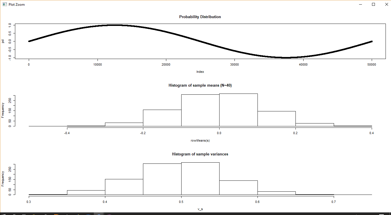
Since the function is nice and symmetric, a value of N=40 is more than enough to result in a sample mean that’s almost equal to the population mean, and the sample mean variance is also almost equal to that predicted by the (known) population variance.

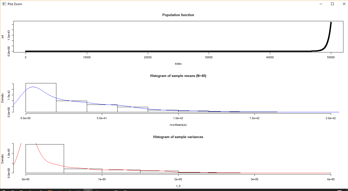
An exponential population

This population is extracted from the exp() function.

1
2

Population:	 Mean = 2202.722807, Variance = 19411026.891557, Variance/N = 485275.672289
Sample Means:	 Mean = 2178.442988, Variance = 467492.546106

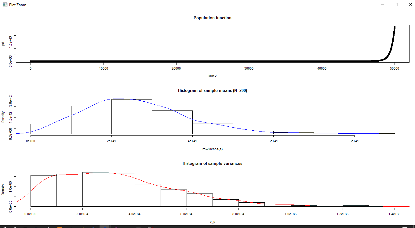
The results are not as perfect as before, but it’s still pretty close. Increasing the parameter of the exponential function from 10 to 100 will result in a plot that’s clearly not normal. Increasing N to 200 brings us closer to CLT expectations.

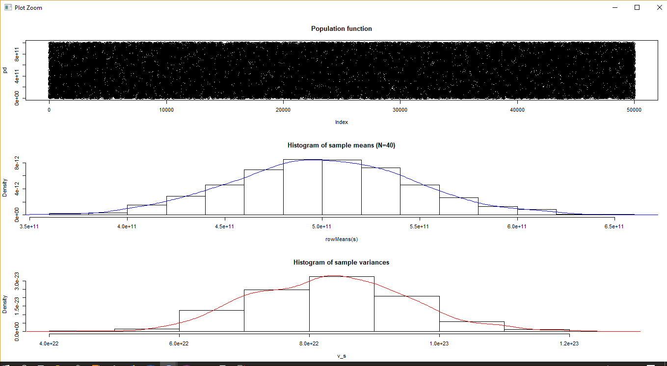
A random function

To illustrate that the CLT does not depend on the original population distribution, we set the population to be a random function. One can see that for a random data, N = 40 is pretty good.

Other considerations

Sampling with and without replacement

The examples are all based on samples taken with replacement, meaning that every sample is drawn from a population of P = 50000, and the samples taken are not deleted from the population. If you reduce the size of the population as you take samples, then the CLT formula needs a correction in the variance formula as specified here. However this can be ignored if the population size is much larger (20x) of the sample size.

Random data

It’s important that you take random data for each of the samples, otherwise you won’t get the desired results. For instance imagine that you keep on repeating the same sample of data, in this case you may never reach close to the population mean until N becomes almost as large as the population. In practice this is a difficult requirement to get right because you might unknowingly introduce biases. For example if you do an online survey as a means of sampling, you might only be targeting a certain segment (eg: tech savvy people) of the population which might invalidate your results with respect to other segments of the population.

Conclusion

That concludes the introduction to CLT. A lot of statistics tests introduce CLT using probability concepts, however CLT - as you can see - is a property of the sums of random numbers and does not require a background of probability.

All the plots I have generated show sampling distribution of variances (in addition to the mean) - this does not follow the normal distribution but instead follows the chi-squared distribution with N degrees of freedom, though to be honest, I can’t visually tell a huge difference.

References

1. CLT
2. Chi-squared distribution
3. A basic statistics course
4. Intuitive CLT