Recently I had the opportunity to play around with some ecological data for statistical analysis using the R programming language. As I didn’t know anything about ecology (or R), I got to learn a bunch of new stuff, and realized that it’s actually very interesting. This post will talk about what I learnt and also serve as an introductory tutorial for someone else getting into stuff like this. However, do note that I’m not an ecologist or a data scientist, so the usual disclaimers apply - if you discover any errors please point them out.

This is the first article and will talk about the basics and species richness and diversity. Further articles will deal with Multivariate and Univariate analysis.

Software of the trade

A fair amount of proprietary software packages for ecological data analysis seem to be available, with PC-ORD, Canoco and PRIMER supposedly being the most popular. A larger list is available here. Luckily for us there are several FOC R packages that can do most of what the proprietary packages do, with greater flexibility. In the R universe, the most important package is vegan.

There is another wrapper package called BiodiversityR that wraps vegan and other stuff to present a GUI interface that allows you to quickly do any fancy test you want. It also comes with an excellent user manual that’s accessible to muggles. Given this, the best workflow is to experiment with the BiodiversityRGUI() and then eventually write your own scripts that natively access vegan APIs for better control over the plotting and parameters for the final publication worthy results.

With regards to species diversity and richness estimation SpadeR is another useful package. It comes with an online version that users who don’t know how to use R can use. EstimateS is standard proprietary software specializing in diversity and richness estimation.

Inputs

Samples and the Species / Environmental Matrix

Generally after you’ve designed your experiments and collected data in the forest or sewer, identified the species you discovered and measured the environmental conditions you’ll be left with two tables of data. The most important one is called the species matrix and this tells you what species you discovered, in what quantity (aka abundance) every time you took a “measurement”. Each “measurement” is called a sample in literature, and typically you’re going to have samples separated across location and/or time. The term sample was a bit confusing to me as coming from a signal processing background I thought it meant each individual species sample. However it doesn’t, and ecologically speaking if you go down to your neighbor’s pond today and come back with a fistful of fish, then that’s one sample. If you do that again tomorrow, that’s another sample.

The species matrix is by convention a series of species samples, with each sample assigned to a new row. The columns are the abundance of each species. All software programs expect such an arrangement by default.

Now in addition to the abundance information you are probably also interested in knowing about how other “factors” (or independent variables) effect the abundance or existence of various species. These “factors” could be environmental (like temperature, pressure..) or not (like location, your collection method..), quantitative (anything that can be assigned a numeric value) or not (like the name of the gardener at each site). These are all recorded in the environmental matrix, and you need to have an entry for each sample in the corresponding species matrix.

Example Analysis

We use some contrived data to illustrate the concepts.

The Accumulation table is:

The corresponding “environment” table:

The Uneven set of samples show a skew with species A being dominant and the rest of the species even at 1 individual each. The Even dataset has an even abundance, the Random set has varying abundance and the Low dataset has the smallest total number of individuals.

The following commands load the test abundance and environment data

1
2
3
4
5
6
7

# Load the BiodiversityR UI
library(BiodiversityR)
BiodiversityRGUI()

# Load data
spa.dummy = read.csv('C:/Users/gov/Google Drive/Zoology/species-dummy.csv', header=TRUE)
env.dummy = read.csv('C:/Users/gov/Google Drive/Zoology/env-dummy.csv', header=TRUE)

Species Richness and Diversity

Species richness is a scalar number to illustrate the variety of species available in an area. Introducing this measure immediately creates a problematic question, is a sample with 9 species of 1 individual each + 1 species of 100 individuals equally rich as one with 10 species of 10 individuals each? The solution is to answer yes to this question, and introduce another measure called diversity that takes into account the relative abundance in addition to the richness.

Richness

When calculating richness with small samples of data, you run into two main problems

1. There is a good chance that you haven’t sampled enough to detect all the present species
2. There is likely to be a wide variation in number of individuals you have in the different samples

The second problem can be solved by using rarefaction curves.

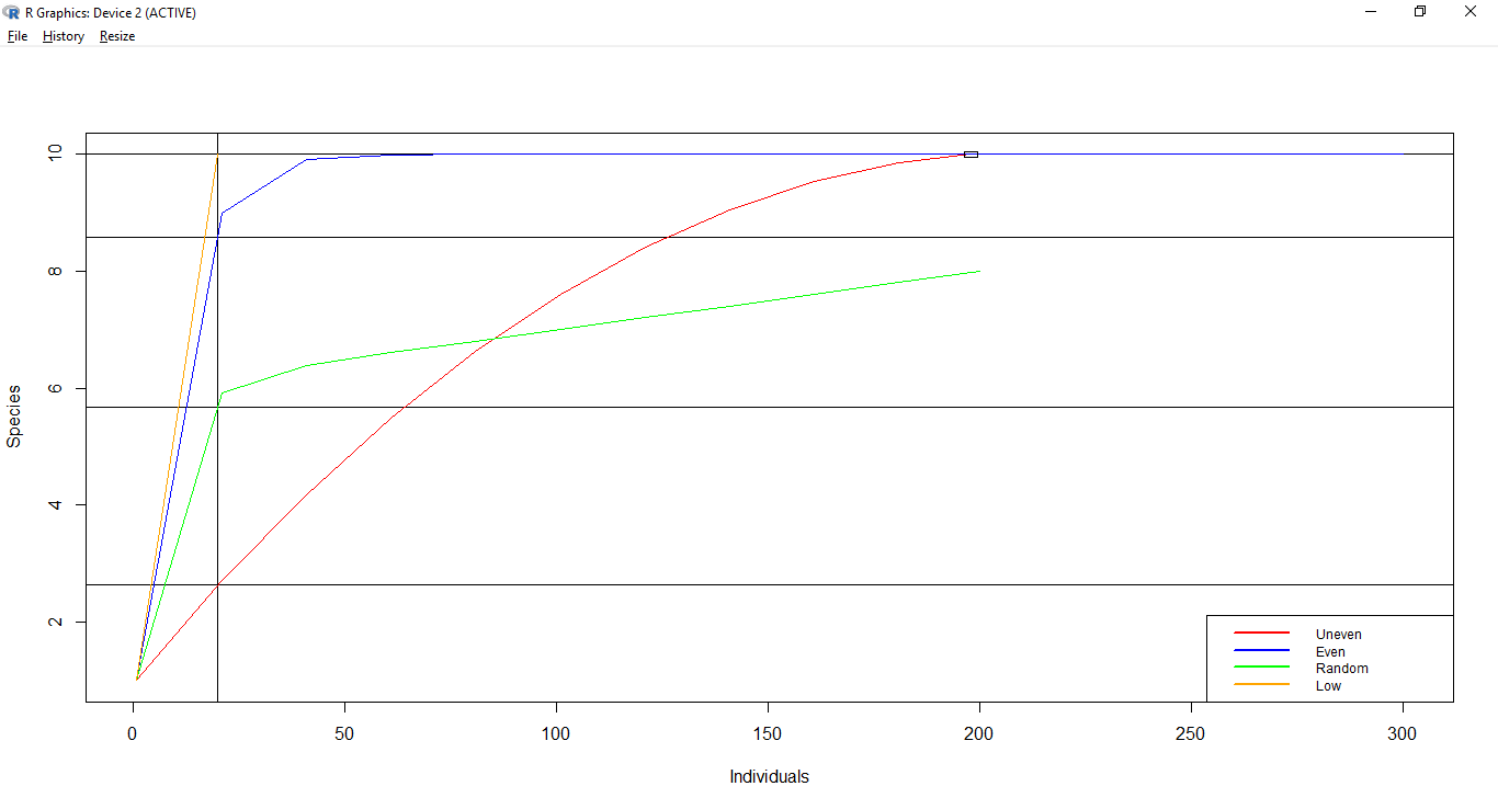
Rarefaction

Rarefaction is an easy graphical approach which involves plotting the species accumulation curve backwards. To plot the curve you take the pooled data and randomly remove an individual / sample and mark the resulting species richness; the process is repeated until you have 0 individuals or samples.

As BiodiversityR does not seem to have a GUI option to plot individual based rarefaction instead of site/sample based, I’m using the vegan commands directly as so:

1
2
3
4
5
6
7
8
9
10
11
12
13
14

# Pool the two samples per community
spa.dummy.pooled = matrix(data = c(colSums(spa.dummy[1:2,]), colSums(spa.dummy[3:4,]), colSums(spa.dummy[5:6,]), colSums(spa.dummy[7:8,])), nrow = 4, byrow = TRUE)

# Calculate lowest number of individuals towards which we must rarefy
raremax = min(rowSums(spa.dummy.pooled))

# Plot
rarecurve(spa.dummy.pooled, step = 20, sample = raremax, col = c("red", "blue", "green", "orange"), xlab = "Individuals", cex = 0.6)
legend("bottomright", legend = c("Uneven", "Even", "Random", "Low"),
	   lty=c(1,1,1,1), # gives the legend appropriate symbols (lines)
	   lwd=c(2.5,2.5, 2.5, 2.5),
	   col=c("red", "blue", "green","orange"), # gives the legend lines the correct color and width
	   cex=0.75 # reduce size of legend box
	   )

To compare communities, you check the species richness for all communities at the point corresponding to the lowest abundance (the vertical line in the plot below). The horizontal black lines correspond to the respective rarefied richness.

Non-parametric richness estimators

Although rarefaction is simple, it’s accuracy is not so obvious. The curve does not predict the eventual species richness, and it’s possible that with more samples the curves may intersect and change in rank; and sampling down means that the lowest sample quantity should be good enough for an accurate deduction. (Apparently this is possible with EstimateS, but I wouldn’t know)

Another class of methods rely on estimating the eventual species richness based on the data you have. Many of them are based on a technique called Good-Turing frequency estimation, which correct the observed richness with estimates of undetected species calculated by looking at the number of singletons/doubletons and low abundance species. The idea being that the existence of singletons etc allude to the fact that you don’t have enough samples and there’s a good chance of discovering more species, where as if you have large abundances for all the species concerned, then your existing data is probably good enough.

There are a bunch of non-parametric methods available called Chao1, Chao2, ACE. All of these can be tried out online using SpadeR and in BiodiversityR. In vegan the specpool() function helps with this.

Calculating the Chao diversity index gives the following result, showing that we expect some new species to be discovered at the Uneven plot while the richness for the Even plot is as calculated from the data without any extra correction.

1
2
3
4
5
6
7
8

Diversity.1 <- diversitycomp(spa.dummy, y=env.dummy, factor1='Type', index='chao' , method='pooled', sortit=FALSE, digits=6)
Diversity.1

Type     n    chao
  Even   2 10.0000
  Low    2 10.0000
  Random 2  9.0000
  Uneven 2 10.0278

Diversity

Next we turn to diversity which takes into account the relative distribution of species (aka evenness) along with the total number of species. The diversity calculated from our data is the diversity at individual spots/samples and is called alpha diversity.

A popular measure of diversity is the Shannon Entropy function invented by Claude Shannon in his Mathematical Theory of Communication. This function measures entropy which is the uncertainty of the process under consideration. If you apply this to an abundance sample, what you get is the uncertainty in species identity - i.e. if you take a random individual from the sample, how confidently / easily can you guess that it belongs to a particular species X. The function attains it’s highest value when all species are equally probable (i.e. the species distribution is perfectly even).

When the diversity is evenly distributed, the equation reduces to

Because of the log here you have to be a bit careful when comparing communities using this index directly, for example (using the base 10 logarithm) if you have two communities with evenly distributed species (for simplicity), one with 10 evenly distributed species and the other with 100, the two communities will have an entropy of 1 and 2 respectively, even though intuitively you would expect the second community to be 10x more diverse than the first one. To fix this problem, one can transform the Shannon Index by taking the inverse logarithm of the index. For a given diversity index this is equivalent to finding the diversity of a community with the same diversity index but with a perfectly evenly distributed population. This technique is applicable for other diversity indices too as is detailed here based on the earlier work by Hill here

Therefore to summarize, it’s helpful to transform the Shannon index to “true diversity” by

This transformed value is also called the first order Hill Number.

The Shannon Diversity for our test dataset shows that - as expected - the Even and Low dataset is the same and higher compared to the other two datasets. BiodiversityR does not seem to have an option for Hill Numbers, so you’ll have to calculate it separately.

1
2
3
4
5
6
7
8

Diversity.1 <- diversitycomp(spa.dummy, y=env.dummy, factor1='Type', index='Shannon' , method='pooled', sortit=FALSE, digits=6)
Diversity.1

Type     n  Shannon
  Even   2 2.302585
  Low    2 2.302585
  Random 2 1.756506
  Uneven 2 0.480094

The classical Shannon diversity index suffers from the same problem as that of the simple richness measures - unknown species. A similar correction factor can be introduced as per Chao et al.. You can experiment with this using SpadeR.

Rank-abundance Curves

Another alternative to the above method of calculating a single numeric number to represent the diversity of a place is to analyze diversity visually. A simple rank abundance curve can show you both the richness and evenness - curves with more species extend longer and those with better evenness are more “horizontal” in nature.

The rank abundance curve of the test data clearly shows the unevenness of the Uneven and Random data points in contrast to the Even and Low datasets.

References

• An excellent overview of richness and diversity measures along with details on plotting Diversity profile is in Anne Chao’s paper here and also here

• Applications to microbial diversity is illustrated here.

• Simplified version of Shannon’s paper - Information theory for intelligent people

• The books - Measuring Biological Diversity and Biological Diversity - frontiers in measurement and assessment by Anne E. Magurran provide an in-depth treatment of biodiversity indicators